
Performance Profile Benchmarking Tool
Published:
The Dolan-More Performance Profile is a method used for comparing the performance of algorithms.
It was popularized by Elizabeth Dolan and Jorge More in their paper titled “Benchmarking Optimization Software with Performance Profiles” (Mathematical Programming, 2002). The performance profile is a way to summarize and visualize the performance of different algorithms across multiple problem instances. It is very much used in the field of mathematical optimization with nearly 5,000 citations of Dolan & Moré, 2002 listed on Google Scholar at the time of writing.
While the method is often associated with Dolan and More, it’s essential to acknowledge the historical roots of performance ratio usage, dating back to at least 1996 with the work of André L. Tits and Yaguang Yang. This historical context highlights the method’s evolution and widespread adoption over the years.
The primary purpose of a performance profile is to assess and compare the effectiveness of a group of solvers on a defined test collection, utilizing a chosen metric or cost. This assessment is shown in a graph that displays the cumulative distribution function of a performance ratio for each algorithm on every problem instance.
How It Works
While traditional benchmarking efforts often involve extensive tables displaying solver performance on various metrics, they face inherent challenges. The sheer volume of data in tables becomes overwhelming, especially for large test sets, and the interpretation of results from these tables frequently leads to disagreements.
The advantage of using performance ratios lies in their ability to offer insights into the percent improvement of a solver’s metric compared to the best solver, while mitigating the impact of a small subset of problems to dominate the conclusions.
To understand how the performance profile works, let’s break down the process. Benchmarks are generated by running a set of solvers ($S$) on a set of problems ($P$), measuring a chosen metric (e.g., CPU time) $t_{p,s}$ for each solvers $s \in S$ applied to problems $p \in P$. It is essential to note that the selected cost metric must be a positive value, where smaller values indicate better performance.
The performance ratio $r_{p,s}$ of solver $s \in S$ on problem $p \in P$ is defined as the ratio of the solver’s metric to the minimum metric among all solvers for that problem, in other words: \(r_{p,s} := \frac{t_{p,s}}{\min_{s \in S} t_{p,s}}\) where $t_{p,s}$ is the value of the chosen metric of solver $s$ on problem $p$, e.g., the CPU time for solver $s$ to solve the problem $p$. Note that the ratio $r_{p,s}$ is greater or equal to $1$. If the chosen metric is possibly 0 then the denominator should be shifted by a small value.
When the solver fails to solve a problem and triggers an alternative stopping criterion, such as reaching a maximum time or iteration limit, we assign a penalty value, usually $+\infty$.
The performance profile is then defined via the cumulative distribution function for the performance ratio $\rho_s:\mathbb{R} \rightarrow [0,1]$ such as \(\rho_{s}(\tau) := \frac{1}{n_p} \sum_{p \in P} 1_{r_{p,s} \leq \tau},\) where $n_p$ is the number of problems, and $1_X$ is the indicator function.
In words, it means the quantities $\rho_s(\tau)$ represents the percentage of problems that, for solver $s \in S$, a performance ratio $r_{p,s}$ is within a factor $\tau$ of the best possible ratio across all problems.
Note that by definition $\rho_s(\tau)$ is always between 0 and 1 and offers valuable insights:
- The values $\rho_s(1)$ gives the percentage of problems where solver $s$ achieved the best ratio. Note that the sum of these percentages across all solvers may exceed 100% in the case of ties.
- The function $\tau \rightarrow \rho_{s}(\tau)$ is a non-decreasing function.
- All solvers should attain a performance ratio of $1$ for $\tau$ sufficiently large unless some of the problems were not solved. In other words, all the solvers will reach a “plateau” representing the percentage of problems solved.
Advantages
- Comprehensive Comparison: The performance profile offers a comprehensive way to compare the performance of multiple algorithms across a diverse set of instances.
- Visual Representation: The graphical representation of the performance profile is easy to interpret. Researchers can quickly identify which algorithms are more competitive by examining the shape and position of the cumulative distribution functions.
- Instance-Specific Assessment: By considering the performance ratio on a per-instance basis, the performance profile allows to identify algorithms that consistently perform well across a range of problem instances. This is especially important in optimization, where the characteristics of instances can vary widely.
- Robustness Analysis: The profile is useful for assessing the robustness of algorithms. Algorithms that exhibit consistent good performance across a variety of instances will have performance profiles concentrated towards the left, indicating reliability. In Dolan & Moré, 2002, the authors justify that performance profiles are relatively insensitive to changes in results on a small number of problems and that they are also largely unaffected by small changes in results over many problems.
- No Need for Aggregation: Unlike some other performance metrics that require aggregating results over instances, the performance profile considers the performance of algorithms on each instance individually, providing a more nuanced evaluation.
- Instance-Specific Insights: Researchers can gain insights into the types of instances where certain algorithms excel or struggle, helping to identify algorithmic strengths and weaknesses in specific problem scenarios.
Disadvantages
- Dependency on Problem Instances: The performance profile is sensitive to the choice of problem instances. Including a diverse set of instances is crucial, and the results can be influenced by the selection of these instances.
- Metric Sensitivity: The performance profile is based on performance ratios, and the choice of the performance measure can impact the results. Sensitivity to the choice of the objective function or metric is a consideration.
- Interpretation Challenges: While the visual representation is generally intuitive, interpreting performance profiles can be challenging when dealing with a large number of algorithms and instances. Researchers need to carefully analyze the plots to draw meaningful conclusions.
- Dependence on Parameter Settings: The performance of optimization algorithms can be sensitive to parameter settings. The performance profile may not fully capture the impact of parameter tuning, and additional analysis may be needed. Finally, the benchmark should be run with similar stopping criteria for all the solvers.
- Limited to Relative Comparison: The performance profile is primarily designed for comparing algorithms relative to each other. It doesn’t provide an absolute measure of algorithm performance, and researchers may need to complement it with other metrics for a more complete assessment.
Implementations
Several online implementations facilitate the generation of performance profiles for mathematical optimization software. Perprof-py is a notable Python package designed for this purpose, offering compatibility with TikZ and matplotlib for graphical output. Additionally, the Julia programming language boasts two significant contributions in this domain: BenchmarkProfiles.jl and SolverBenchmark.jl. These Julia packages provide effective tools for creating performance profiles and contribute to the growing availability of resources for benchmarking and comparing optimization algorithms. Researchers and practitioners in the field can leverage these implementations to assess the performance of solvers and gain valuable insights into algorithmic behavior across diverse problem instances.
Performance Profile Interpretation
In the realm of performance profiles, Dolan and Moré’s 2002 article provides examples that shed light on the interpretation of performance profiles within extensive benchmarks.
We delve further into the analysis with additional examples aimed at illustrating diverse situations and their nuanced interpretations. Throughout the following examples, we place a particular emphasis on the interpretation of performance profiles, offering readers practical insights into understanding and analyzing results. These examples span various scenarios, showcasing the adaptability of performance profiles in capturing different facets of solver performance across distinct benchmarks.
Additionally, it is essential to note that, in all the forthcoming examples, an unsolved problem is designated with a metric value of $+\infty$.
Example 1: A clear winner
We consider here two solvers on a set of 5 problems.
using BenchmarkProfiles, Plots
T = [
  1.0 5.0;
  1.0 10.0;
  1.0 15.0;
  1.0 20.0;
  1.0 20.0;
]
performance_profile(PlotsBackend(), T, ["Solver A", "Solver B"])
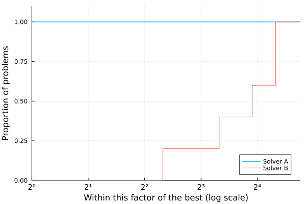
We can observe from this profile that:
- Solver A was better than Solver B on all problems;
- Solver A and Solver B both solved all the problems. Therefore, it is clear that on this test set and according to the chosen metric Solver A is preferable.
Example 2: Fast but not robust
We consider here two solvers on a set of 8 problems.
using BenchmarkProfiles, Plots
T = [
  1.0 5.0;
  1.0 10.0;
  1.0 20.0;
  5.0 10.0;
  7.0 15.0;
  6.0 5.0;
  Inf 20.0;
  Inf 20.0;
]
performance_profile(PlotsBackend(), T, ["Solver A", "Solver B"])
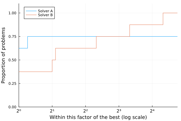
We can observe from this profile that:
- Solver A is better than Solver B on 62% of the problems;
- Solver B solves 75% of the problems within a factor $\approx 2^3$ of the best solver, and all the problems within a factor $\approx 2^5$;
- Solver B solves all the problems, while Solver A only solves 75% of the problems.
Therefore, we can observe a mixed situation here. If one is interested in solving efficiently 75% of the problems, then Solver A is of choice. Howeover, Solver B is more robust as it mangages to solve all the problems.
Example 3: Very small factor
The following exemple shows that we need to pay attention to the factors on the x-axis.
using BenchmarkProfiles, Plots
T = [
  1.0 1.0003;
  1.0 1.0003;
  1.0 1.0003;
  1.0 1.0003;
  1.0 1.0003;
]
performance_profile(PlotsBackend(), T, ["Solver A", "Solver B"])
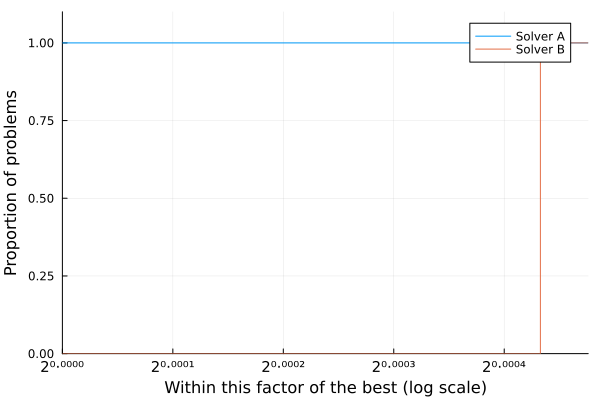
In this case, it is clear that Solver A is better than Solver B, however the factor of difference is so small that it is difficult to draw a clear line between both. This is a situation where either both solvers are equivalent or the metric chosen is not appropriate.
The difficult case of more than 2 solvers
The following example was taken from Gould & Scott, 2016 where is shown the performance of three solvers on a test set of five problems, where the smaller the statistic, the better the solver performance.
| Problem | Solver A | Solver B | Solver C |
|---|---|---|---|
| 1 | 2 | 1.5 | 1 |
| 2 | 1 | 1.2 | 2 |
| 3 | 1 | 4 | 2 |
| 4 | 1 | 5 | 20 |
| 5 | 2 | 5 | 20 |
using BenchmarkProfiles, Plots
T = [
  2.0 1.5 1.0;
  1.0 1.2 2.0;
  1.0 4.0 2.0;
  1.0 5.0 20.0;
  2.0 5.0 20.0;
]
performance_profile(PlotsBackend(), T, ["Solver A", "Solver B", "Solver C"])
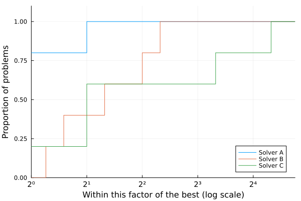
Solver A is the best on 80% of the problems in the test set, Solver B is not the winner on any. Moreover, Solver A solves all the problems within a factor 2 of the best. Thus, it is the most preferable choice over Solver B and Solver C.
Focusing on Solver B and Solver C: if we are interested in having a solver that can solve at least 60% of the test problems with the greatest efficiency then Solver C seems preferable to Solver B.
Trying to confirm this statement and reproducing the performance profile without Solver A however is showing a different story.
using BenchmarkProfiles, Plots
T = [
  2.0 1.5 1.0;
  1.0 1.2 2.0;
  1.0 4.0 2.0;
  1.0 5.0 20.0;
  2.0 5.0 20.0;
]
performance_profile(PlotsBackend(), T[:,2:3], ["Solver B", "Solver C"])
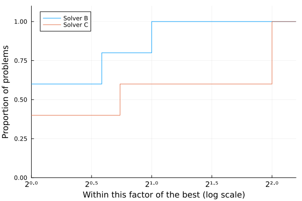
When comparing two solvers on a given test set, performance profiles give a clear measure of which is the better solver for a selected range. But as the examples above illustrate, if performance profiles are used to compare more than two solvers one cannot directly establish a ranking. The article Gould & Scott, 2016 also contains more realistic examples of such phenomenon.
Profile with more metrics and profile wall
One of the drawback of performance profile is the sensitivity to the chosen metric. A straightforward extension is to consider more than one merit function. The following illustration is selected from the article Migot et al., (2022). DCISolver.jl: A Julia Solver for Nonlinear Optimization using Dynamic Control of Infeasibility. Journal of Open Source Software, 7(70), 3991.
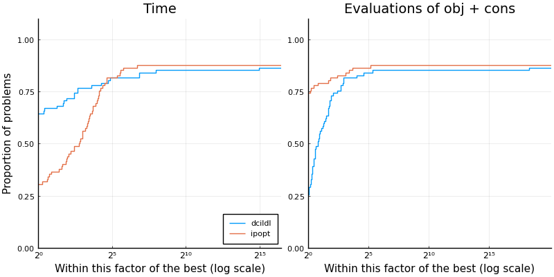
This performance profile compares DCISolver.jl variant LDL against Ipopt on 82 nonlinear continuous optimization problems. It uses two merit functions: the elapsed time to solve a problem, and the number of evaluations of objective and constraint functions. This latter quantity is sometimes used to be independent of the evaluation and the implementation adaptation on the computer, while still being strongly correlated to the elapsed time.
Ipopt solved 72 problems (88%) successfully, which is one more than DCI. The plot on the left shows that Ipopt is the fastest on 28% of the problems, while DCI is the fastest on 72%. The plot on the right shows that Ipopt used fewer evaluations of objective and constraint functions on 70% of the problems, while DCI used fewer evaluations on 24%. Since, it doesn’t add up to 88%, there was a tie in the number of evaluations on 6%.
Overall, this plot tends to show that DCI variant LDL is good implementation as it fast, however it uses more evaluations which can be problematic depending on the modeling tool used to access objective and constraint functions.
It is possible to extend this benchmark to more solvers. The following illustrates a similar benchmark where a third solver is added, KNITRO. The first pair of profile is similar to what has been discussed before. The other profiles are showing two-by-two profiles in order to overcome the difficulty raised earlier.
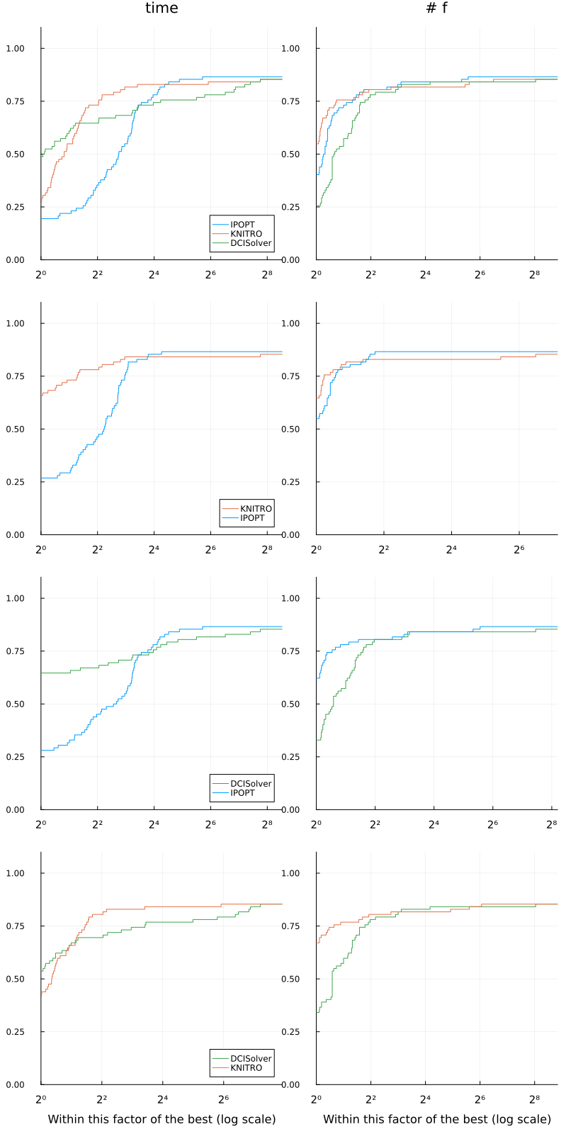
This type of profile wall allows to build more concrete conclusions on the strenght of each solvers.
More on benchmarks
Performance profiles use a performance ratio instead of relying on the count of function evaluations needed to solve a problem. Consequently, performance profiles do not provide the percentage of problems that can be successfully addressed (within a specified tolerance, $\tau$) based on a particular quantity of function evaluations. This data, which is crucial for users dealing with resource-intensive optimization problems and who are keenly interested in the immediate performance of algorithms, is, however, supplied by the data profiles More & Wild, 2009.
References
Dolan, E. D., & Moré, J. J. (2002). Benchmarking optimization software with performance profiles. Mathematical programming, 91, 201-213. DOI: 10.1007/s101070100263
Gould, N., & Scott, J. (2016). A note on performance profiles for benchmarking software. ACM Transactions on Mathematical Software (TOMS), 43(2), 1-5. DOI: 10.1145/2950048
Moré, J. J., & Wild, S. M. (2009). Benchmarking derivative-free optimization algorithms. SIAM Journal on Optimization, 20(1), 172-191. DOI: 10.1137/080724083
Siqueira, A. S., da Silva, R. G. C., & Santos, L. R. (2016). Perprof-py: A python package for performance profile of mathematical optimization software. Journal of Open Research Software, 4(1), e12-e12. DOI: 10.5334/jors.81
Tits, A. L., & Yang, Y. (1996). Globally convergent algorithms for robust pole assignment by state feedback. IEEE transactions on Automatic Control, 41(10), 1432-1452. DOI: 10.1109/9.539425